Thousands of lines of hand-written CUDA C++, now Python. Less code, and it runs faster.

A single collision event in a particle detector holds a variable number of particles, each with a variable number of measurements:

[[1.1, 2.2, 3.3], [], [4.4, 5.5]]

Awkward Array is a Python library for manipulating nested, variable-length (“ragged”) data like this with NumPy-like idioms. It stores that data flat, as one content buffer holding every value contiguously plus an offsets array marking where each sublist begins and ends:

content:  [1.1, 2.2, 3.3, 4.4, 5.5]
offsets:  [0, 3, 3, 5]        # the empty middle list spans no elements

Nothing is wasted on padding, but every operation must then be written in terms of those two buffers rather than a simple shape. That is where dense GPU tensor frameworks stop helping: they want rectangles. For several years, Awkward’s answer was a dictionary of hand-written CUDA C++ kernels compiled at runtime with CuPy.

The Awkward Array and NVIDIA teams have now rebuilt that layer on cuda.compute, which brings the CUDA C++ parallel-algorithm libraries CUB and Thrust (the reductions, scans, and sorts that power production GPU software) into Python as ordinary callables. Instead of writing a kernel, the backend now composes ones that already exist. Four results stand out.

1. The GPU code is Python now#

ak.min, the minimum over each ragged sublist, took three kernel launches in CUDA C++: initialize a scratch buffer, reduce within each block using shared memory and explicit thread synchronization, and copy the result out. Each communicated with the next through global memory.

It is now a single call to a library primitive:

import cupy as cp, numpy as np
from cuda.compute import OpKind, segmented_reduce


def awkward_reduce_min(
    toptr: cp.ndarray,
    fromptr: cp.ndarray,
    offsets: cp.ndarray,
    outlength: int,
    identity: float,
) -> None:

    toptr[:outlength] = identity
    segmented_reduce(
        fromptr,
        toptr,
        offsets[:-1],
        offsets[1:],
        OpKind.MINIMUM,
        np.asarray(identity, dtype=fromptr.dtype),
        outlength,
    )

segmented_reduce performs one reduction per segment, and offsets[:-1] and offsets[1:] hand it the start and end of each sublist directly. No CUDA C++, no synchronization, no scratch buffers: the library handles all of it.

Awkward’s user-facing API is unchanged. Underneath, 2.10.0 routes 106 of its 133 GPU kernels (80%) through cuda.compute, up from none in 2.8.11. Every reduction and the sort now run through it with no hand-written implementation remaining. The 27 still in CUDA C++ handle structural work like jagged indexing, padding, and validity checks. Their control flow depends on the ragged layout itself, which fits the segmented primitives less naturally. That migration is ongoing. Counting only code that must actually be maintained, the switch to cuda.compute has so far cut hand-written CUDA C++ from 8,288 lines to 2,170 — a 74% reduction.

2. The abstraction made it faster#

We might expect to pay something for the abstraction.

Over 5,000,000 ragged sublists, ak.argmin takes 0.96 ms per call as a hand-written CUDA kernel and 0.39 ms through cuda.compute: 2.5x faster, with identical output.

That speedup is inherited rather than hand-tuned, which is exactly the point of building on CUB: segmented reductions are difficult to write well by hand, and CUB’s have been tuned per architecture for years. Awkward gets that tuning now, and the next architecture’s when it ships, without changing its own code.

3. A whole physics formula can collapse into one kernel#

The first two results came from the migration. For this one, a user drops down to cuda.compute and composes the primitives by hand.

Awkward evaluates eagerly: every operation returns a real array, so a chain of them writes an intermediate to global memory at each step and reads it back at the next. cuda.compute algorithms instead accept iterators that are evaluated lazily as the algorithm runs, letting many logical steps ride along inside a single pass. That is kernel fusion, and it saves both the memory traffic and the launch overhead.

Example: di-muon invariant mass#

The opposite-sign di-muon invariant mass, a standard reconstruction in particle physics, combines a few measured quantities for every pair of particles in an event. In Awkward, it is one line:

mu1, mu2 = ak.unzip(ak.combinations(muons, 2))
mass = np.sqrt(
    2 * mu1.pt * mu2.pt * (np.cosh(mu1.eta - mu2.eta) - np.cos(mu1.phi - mu2.phi))
)

Evaluated step by step, that chain of arithmetic and trigonometric operations becomes one or more kernels per step, with every intermediate written out as a full-length array and read back.

Written by hand as one cuda.compute call, the whole formula becomes a single operator: a gpu_struct keeps each particle’s fields together, a ZipIterator combines them, and a PermutationIterator produces each pair on demand. The operator sees one complete pair at a time, and no intermediate is ever built.

Over all such pairs in a CMS open-data sample:

2.5x faster, with nothing allocated in between.

4. At analysis scale, the gap widens#

We ran the ADL benchmark queries (a standard set of physics-analysis tasks) on CMS 2012 open data, against released Awkward 2.8.11 on its hand-written CuPy backend, the last version before cuda.compute. For the two combinatoric queries below, the Awkward expression is unchanged; only the backend underneath differs, so the comparison isolates the migration itself.

Measured on the GPU compute stage at 100k, 1M, and 10M events, both speed up by margins that grow with the data:

• the di-muon reconstruction from section 3: 60x → 422x → 3634x
• a second combinatoric query: 45x rising to 250x

cuda.compute’s time stays approximately constant across those sizes while the hand-written implementation grows super-linearly, so the gap widens as data grows rather than closing.

The result that isn’t a number#

A stated goal of the Awkward Array project is to let physicists and data analysts write high-performance code in Python without GPU expertise. The old backend required contributors to understand CUDA thread hierarchies, atomics, and shared-memory behavior before they could add or fix a kernel. The new one asks for an ordinary Python function and a call to the right primitive. Domain scientists can read it, review it, and unit-test its logic without a GPU.

Awkward knows the problem. cuda.compute knows the hardware. The result is Python that’s simpler and faster than the CUDA C++ it replaced.

Full methodology, per-query results, and the code-counting rules are in “GPU-Accelerated Awkward Arrays with CUDA Python” by Ashwin Srinath (NVIDIA) and Ianna Osborne (Princeton University), Proceedings of the 24th Python in Science Conference (SciPy 2026). All measurements were taken on an NVIDIA RTX PRO 6000 Blackwell Server Edition with CUDA 13.2, cuda.compute 1.1.0, and CuPy 14.1.1; every benchmark was run twice on independent machines, with structural counts identical and timings agreeing to within a few percent. Migration progress is tracked in scikit-hep/awkward#3793.

Much of the kernel migration was implemented by Maxym Naumchyk. Thanks also to the cuda.compute and CUB/Thrust developers at NVIDIA and to the Scikit-HEP community. This work was supported in part by NSF grants OAC-1450377, OAC-1836650, OAC-2103945, PHY-2121686, and PHY-2323298.

In particle or high energy physics (HEP), by the time you draw a plot the data are almost always already binned. A long stretch of the analysis pipeline — Uproot, Coffea, boost-histogram, hist — has reduced terabytes of events into a handful of histograms that you now want to display. That single fact bends what a good plotting API for HEP needs to look like, and it is where mplhep — a thin, focused matplotlib wrapper in the Scikit-HEP ecosystem — sits.

This post walks through three things mplhep contributes: a histogram plotting function for pre-binned data, comparison panels (ratio/pull/efficiency) on top of it, and a set of experiment style sheets that match the conventions ATLAS, CMS, LHCb, ALICE and DUNE publications require.

Plotting pre-binned histograms#

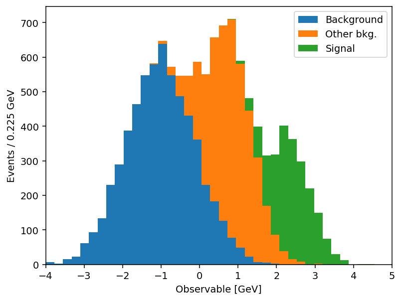
If you want to plot a histogram matplotlib had a great function for it - plt.hist, except in its convenience it not only serves the plotting, but also wraps the histogramming - (counts, edges) from np.histogram. But if the histogram you want to visualize is already made you used to have to either “hack” plt.hist by filling 1’s and passing histogram values as weights, or use plt.step and hack your len(x) = len(y) + 1 input information into the same length or accept plt.bar with its own limitations.

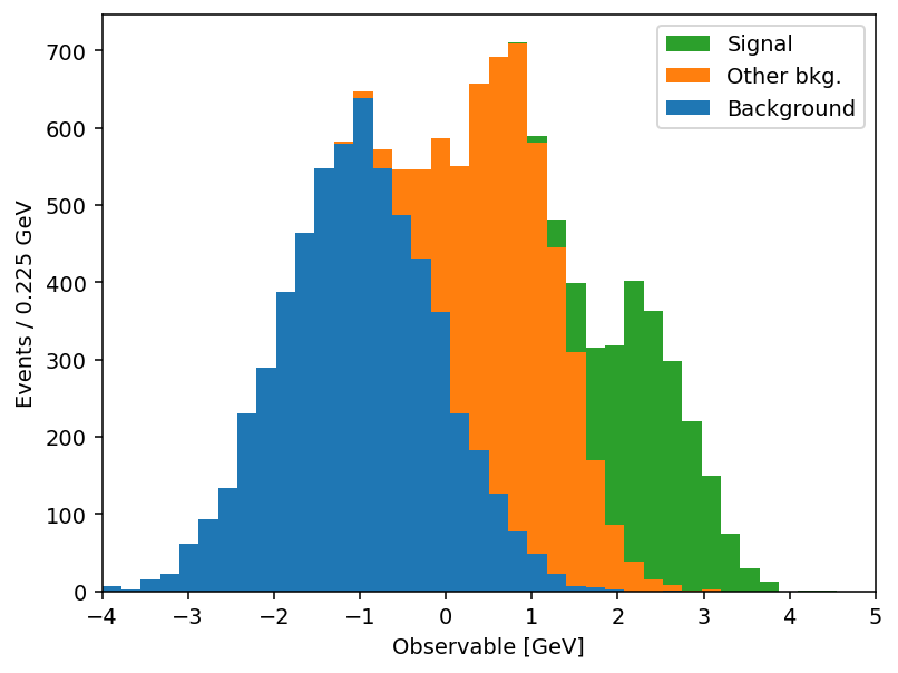
To improve this particular user experience the mplhep authors contributed a new distinct primitive plt.stairs, which was added in matplotlib 3.4 specifically for pre-binned data. This simplifies the syntax for HEP users significantly, but at the same time plt.stairs is still just a primitive function compared to the rich functionality of plt.hist. To mimic and indeed extend this functionality for the needs of particle physicists and indeed anyone who handles pre-binned histograms, we present the mplhep (imported as mh) library with mh.histplot at its core (see also the full docs).

import matplotlib.pyplot as plt
import numpy as np

cumulative = np.zeros_like(ha, dtype=float)
for cnt, lab in zip([ha, hb, hc], labels):
    new = cumulative + cnt
    plt.stairs(new, edges, baseline=cumulative, fill=True, label=lab)
    cumulative = new
plt.legend()

import matplotlib.pyplot as plt
import mplhep as mh

mh.histplot(
    [ha, hb, hc],
    edges,
    stack=True,
    histtype="fill",
    label=labels,
)
plt.legend()

Same output, half the code. And the savings compound once you actually use the keyword arguments. mh.histplot accepts a NumPy tuple, a hist.Hist, a boost_histogram.Histogram, or any object implementing the PlottableProtocol, so the same call works regardless of what your analysis framework hands you. From there, the keywords most analyses lean on:

• yerr=True → Poisson intervals for integer counts; pass a 1D array for symmetric errors, a 2D (2, N) array for asymmetric ones, or yerr=False to suppress them entirely.
• w2=variances → sum-of-weights-squared propagation for weighted MC. When combined with yerr=True, mplhep picks Poisson intervals for integer-like w2 and sqrt(w2) otherwise; w2method= lets you force one or the other.
• sort="yield" → auto-sort a stack by total yield (largest at the bottom); "label" sorts alphabetically; append _r to reverse.
• histtype= → "step", "fill", "errorbar", "bar", "barstep", or "band" (which spans the yerr range — perfect for systematic uncertainty bands without a second call).
• density=True / binwnorm=1.0 → normalise to unit area or per unit bin width.
• flow="show" / "sum" / "hint" → handle under- and overflow bins explicitly.
• blind=(lo, hi) (or mh.loc[lo:hi]) → hide bins in a signal region for blind analyses.

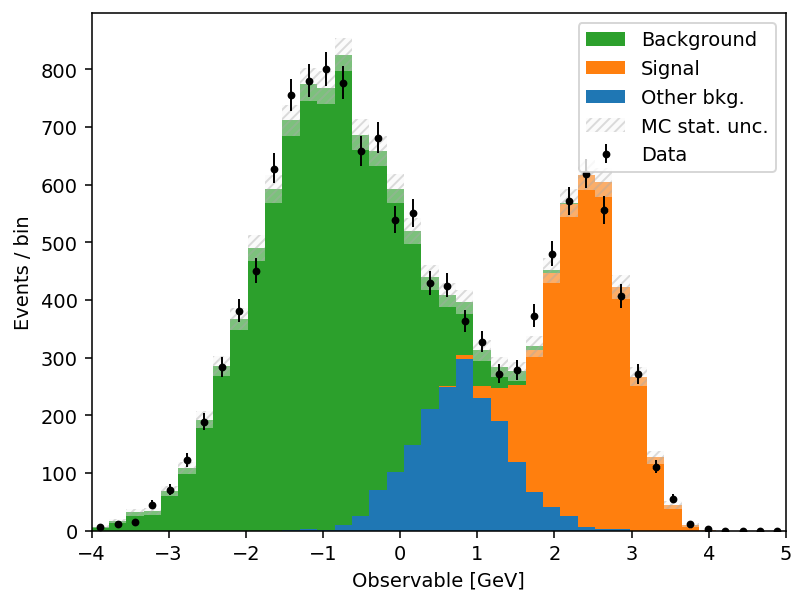
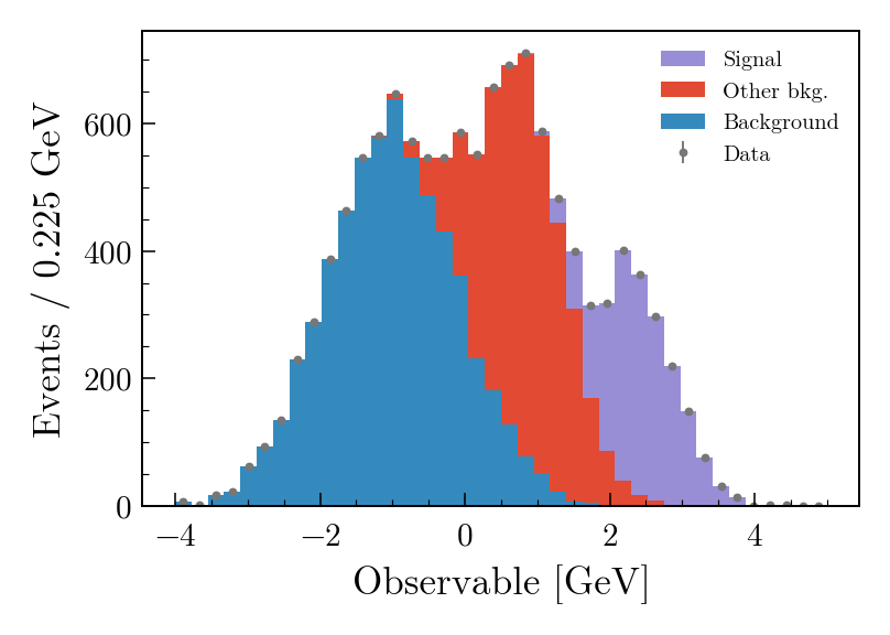
The full list is in the mh.histplot API reference. A short example that exercises several of these — sum-of-weights-squared on a weighted MC stack, auto-sorting by yield, a hatched MC uncertainty band, and Poisson-interval errors on the data overlay:

mh.histplot(
    mc_components,
    edges,
    w2=mc_variances,  # propagate Sumw2 for weighted MC
    stack=True,
    sort="yield",  # smallest yield on top of the stack
    histtype="fill",
    label=["Background", "Other bkg.", "Signal"],
)
mh.histplot(
    mc_total,
    edges,
    yerr=np.sqrt(mc_total_var),
    histtype="band",  # filled band spanning ±yerr
    label="MC stat. unc.",
    color="gray",
    alpha=0.4,
)
mh.histplot(
    data_counts,
    edges,
    yerr=True,  # Poisson intervals for integer counts
    histtype="errorbar",
    color="black",
    label="Data",
)

Stacks and comparison panels#

A HEP plot rarely stops at a single histogram. The canonical figure has a stacked background model, an unstacked signal or systematic-uncertainty band, data points with errors on top, and a thinner comparison panel underneath: a ratio, a pull, an efficiency. Those panels all share a layout — twinned bins, reference line at 1 or 0 — and they’re surprisingly tedious to assemble in matplotlib.

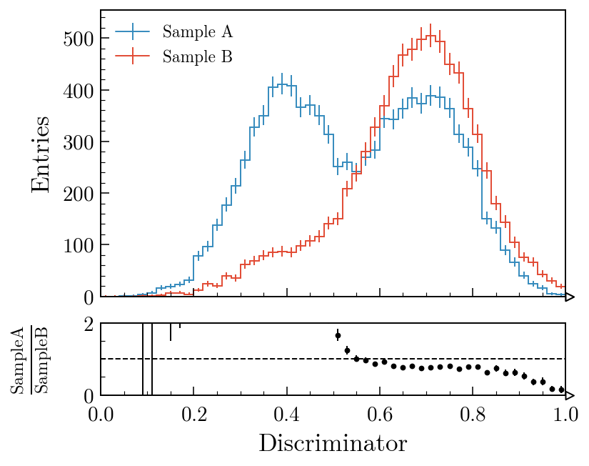
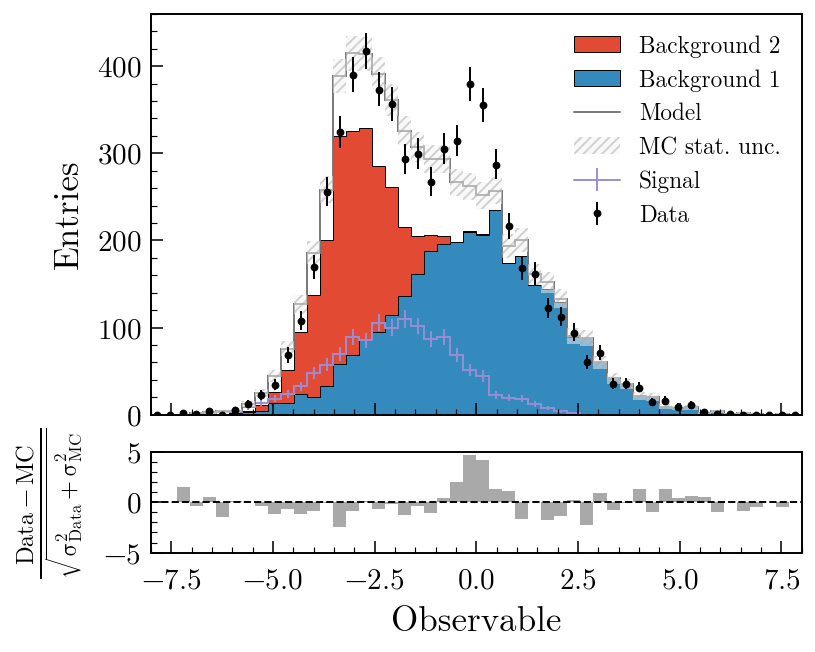
mh.comp.hists builds one in a single call for the two-histogram case; mh.comp.data_model handles the full data-versus-model figure with stacked and unstacked components, MC statistical uncertainty band, and any of the same comparison types in the lower panel:

fig, ax_main, ax_comp = mh.comp.hists(
    h1,
    h2,
    xlabel="Discriminator",
    h1_label="Sample A",
    h2_label="Sample B",
    comparison="ratio",
)

fig, ax_main, ax_comp = mh.comp.data_model(
    data_hist=data,
    stacked_components=[bkg_a, bkg_b],
    stacked_labels=["Bkg 1", "Bkg 2"],
    unstacked_components=[signal],
    unstacked_labels=["Signal"],
    comparison="pull",
)

comparison= also accepts "difference", "relative_difference", "asymmetry" and "efficiency"; the MC statistical uncertainty is propagated through all of them. Swapping "pull" for "ratio" in the second example swaps the lower panel out with no other code changes. The comparisons guide covers every variant with worked examples; the gallery is the fastest way to find a plot that looks like the one you’re trying to make.

Experiment styles#

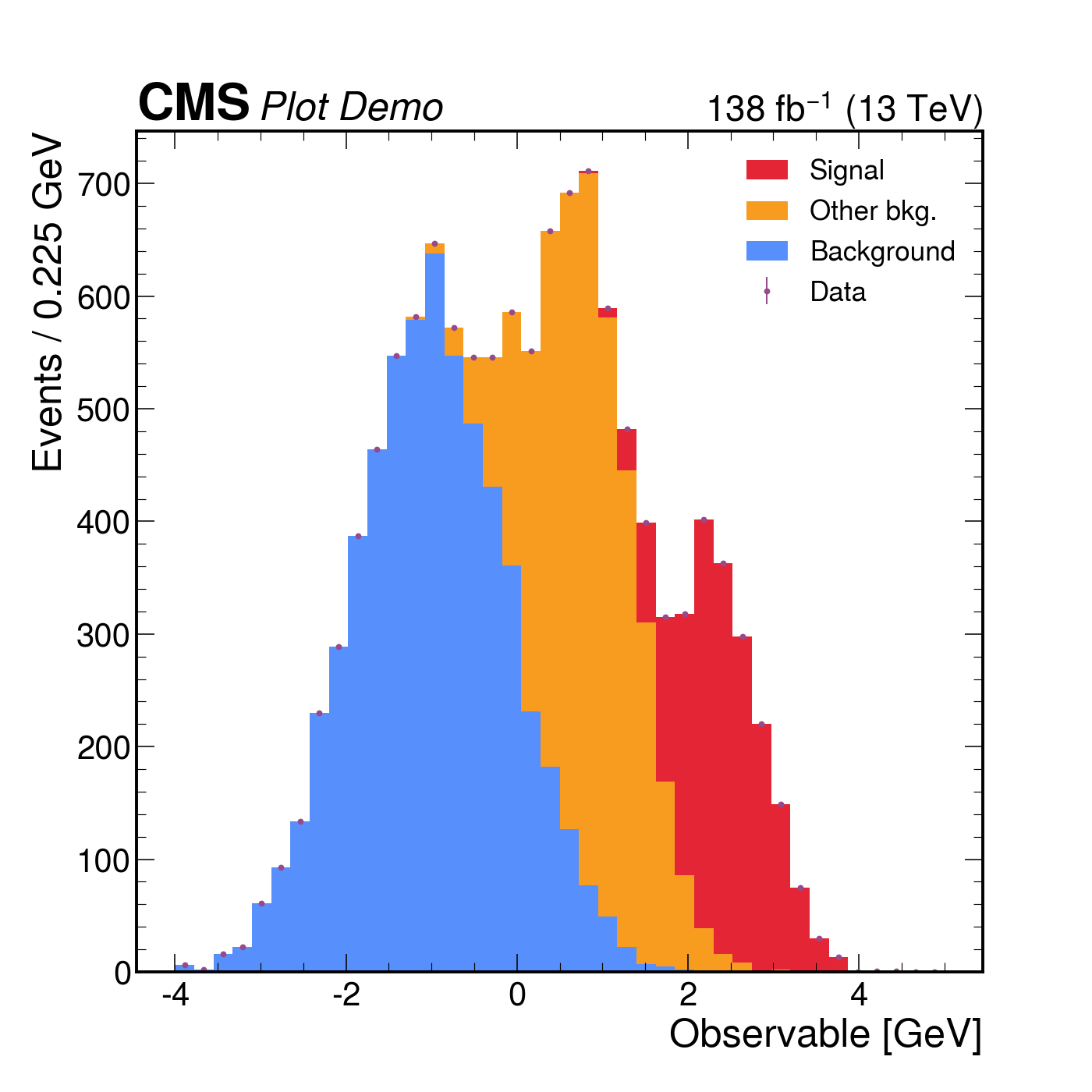
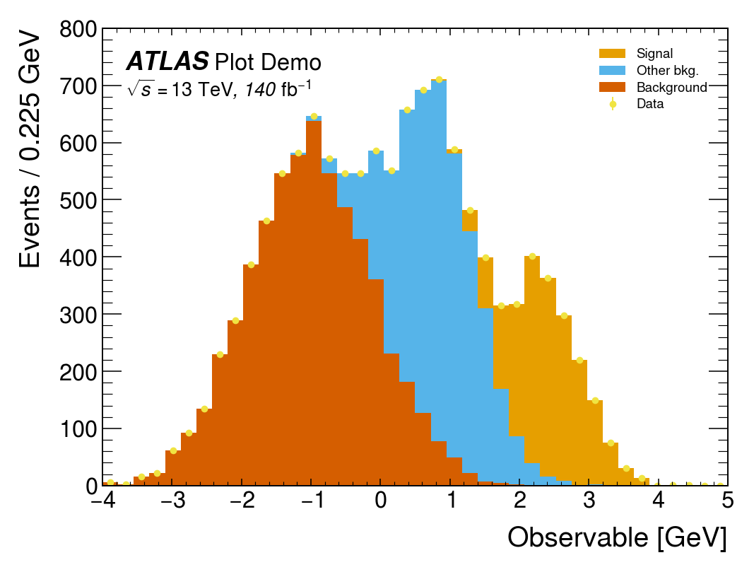
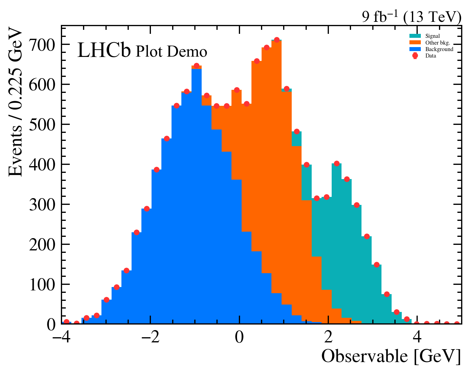
The third thing mplhep does is take care of the typography. Every collaboration has a house style — a font, a “CMS” / “ATLAS” / “LHCb” label with a status qualifier, a √s and integrated-luminosity string, specific tick directions and minor-tick behaviour, a colour cycle. mh.style.use("CMS") (or "ATLAS", "LHCb2", "ALICE", "DUNE") sets matplotlib’s rcParams accordingly and bundles the open fonts (TeX Gyre Heroes as a Helvetica stand-in, Fira Sans, etc.) so the result is reproducible across operating systems. The collaboration tag is placed by a matching helper — mh.cms.label, mh.atlas.label, mh.lhcb.label, mh.alice.label, mh.dune.label — which knows where each one is meant to live (CMS above the axes in the figure margin; ATLAS, LHCb and ALICE inside the axes at top-left). For figures heading somewhere that doesn’t fit a single collaboration’s house style, mh.style.use("plothist") provides a neutral serif look with the same comparison-panel ergonomics and no experiment tag. The styling guide catalogues every available style and the exact arguments each .label() helper accepts.

with plt.style.context(mh.style.CMS):
    fig, ax = plt.subplots()
    mh.histplot(
        [ha, hb, hc],
        edges,
        stack=True,
        histtype="fill",
        label=["Background", "Other bkg.", "Signal"],
        ax=ax,
    )
    mh.histplot(
        ha + hb + hc, edges, histtype="errorbar", color="black", label="Data", ax=ax
    )
    mh.cms.label("Plot Demo", data=True, lumi=138, com=13, ax=ax)
    mh.mpl_magic(ax=ax)

The same three-component stack with data points rendered four ways. Each style picks its own colour cycle, font, and label conventions; mh.mpl_magic auto-grows the y-axis so the experiment tag, legend and data don’t fight for the same space, and is one of a small set of layout helpers (yscale_legend, yscale_anchored_text, sort_legend, append_axes, …) that the utilities guide covers in full.

The same data, the same single mh.histplot call — only the active style context changes.

Where it fits#

mplhep is part of Scikit-HEP, a collection of pure-Python tools for particle physics that also includes hist, Uproot, Awkward Array, vector and pyhf, among many others. It deliberately stays a thin layer on top of plain matplotlib rather than replacing it — every figure mplhep produces is a regular Figure/Axes pair you can keep customising with the matplotlib API you already know. The point is to remove the friction of the conventions, not the flexibility underneath them.

If you work in HEP, pip install mplhep followed by mh.style.use(...) should be the first two lines of any plotting notebook. If you don’t, mh.histplot for pre-binned data and the comparison-panel machinery are still useful well outside the field — anywhere “two histograms and their ratio” is the natural unit of a figure.

• Docs: scikit-hep.org/mplhep — start with the basic plotting, comparisons, styling and utilities guides, browse the gallery for inspiration, or jump to the full API reference.
• Source: github.com/scikit-hep/mplhep
• Discussion: github.com/scikit-hep/mplhep/discussions